Frequency domain analysis converts time-domain signals (raw EEG/MEG data) into the frequency domain to examine the power distribution across different frequency components. This analysis is fundamental for understanding brain oscillations and identifying characteristic rhythms.
Key Concepts
Frequency bands (as defined in NeuroAnalyzer, see band_frq()):
delta: 0.5–4 Hz
theta: 4–8 Hz
alpha: 8–13 Hz
beta: 13–30 Hz
gamma: 30–150 Hz (limited by the Nyquist frequency)
Power spectral density (PSD): how the power of the signal is distributed across frequencies
Peak frequency: the frequency with the maximum power within a band
Band power: the power within a frequency range
Frequency Range and Band Calculations
Getting range of frequencies and Nyquist frequency:
Number of frequencies: 128001
Frequency step:        0.001 Hz
Nyquist frequency:     128.0 Hz
hz is the vector of frequencies of the Fourier transform of the whole signal (1000 seconds, so the frequency step is 1/1000 Hz); nyq is the Nyquist frequency (half of the sampling rate).
Calculating band frequency range:
band_frq(eeg; band =:alpha)
(8.0, 13.0)
Tip: the upper limit of a band is truncated to the Nyquist frequency, e.g. the gamma band (30–150 Hz) becomes 30–128 Hz for this recording (sampling rate 256 Hz). band_frq(eeg; band = :list) prints all available bands.
From time domain to frequency domain
A recorded EEG signal \(x(t)\) is a function of time, but many of its most interesting properties - the alpha rhythm at ~10 Hz, sleep spindles at 12–15 Hz, gamma oscillations above 30 Hz - are defined by frequency. Frequency-domain analysis converts the signal into a representation that shows how much amplitude, power, or energy is present at each frequency.
The bridge between the two domains is the Fourier transform:
where \(X(f)\) is the Fourier transform of \(x(t)\). Strictly speaking, \(\vert X(f) \vert^2\) is the energy spectral density (units: energy per Hz) and is appropriate for finite-energy transients.
For ongoing signals with finite power but infinite energy (like a continuous EEG recording), we instead use the power spectral density (PSD), \(S(f)\), obtained by averaging \(\vert X(f) \vert^2\) over time or over segments:
Spectrum: the amplitude (or magnitude) of the signal as a function of frequency - what frequencies are present and how strong they are.
Spectral density: the distribution of power across the frequency components composing the signal - how the total power is spread out over frequency.
The taper problem
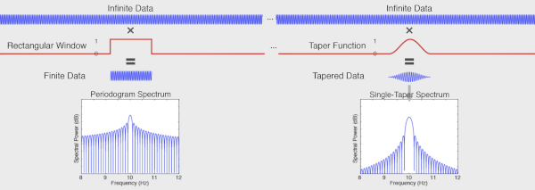
An ideal infinitely long 10 Hz sine has all its power concentrated at a single frequency: the spectral density shows one infinitely sharp peak at 10 Hz.
A two-second 10 Hz sine, however, is mathematically the infinite sine multiplied by a rectangular window (a “taper”) that turns the signal on and off. In the frequency domain, multiplication becomes convolution, so the resulting spectrum is the ideal delta peak convolved with the spectrum of the rectangle - which spreads energy across many frequencies, with a peak at 10 Hz.
The rectangular taper has its own spectrum, with a broad main lobe and a series of side lobes caused by the abrupt transitions at its edges (the sharper the edge, the more high-frequency content).
Because we can never record forever, every real spectrum is computed through a window. This makes the periodogram a biased spectral estimator: it always deviates from the ideal spectrum, and the deviation is worst for short signals.
The bias comes in two flavors:
Bias type
Cause
Consequence
Narrowband bias
width of the main lobe
blurs peaks that are close together; sets the frequency resolution - the minimum separation at which two peaks can be distinguished
Broadband bias
side lobes
spectral leakage: energy from a strong frequency component “leaks” into distant frequency bins, masking or contaminating weaker components
Solution: use a smoother taper, e.g. a Hanning (Hann) taper. Tapers trade the two biases against each other:
Hanning tapers off smoothly to zero at the edges → dramatically smaller side lobes → less broadband bias (less leakage).
But the main lobe is wider → increased narrowband bias (poorer frequency resolution).
Smaller side lobes reveal frequency peaks that would otherwise be hidden inside the leakage of a stronger neighboring peak.
Common tapers:
Taper
Side lobes
Main lobe width
Typical use
Rectangular (boxcar)
highest (−13 dB first lobe)
narrowest
avoid for spectral estimation
Hanning / Hamming
low (−31 / −43 dB)
~2× rectangular
general-purpose single-taper analysis
Gaussian
very low
wide
smooth, well-localized spectra
Slepian (DPSS)
optimized
controllable bandwidth
multitaper analysis
Methods of estimating power
Power spectrum shows the strength (power) of the signal at each component frequency - it converts the signal from the time domain to the frequency domain. Because we estimate it from finite, noisy data, many estimators exist, all trading variance against bias (resolution):
Welch periodogram - average periodograms of overlapping, tapered segments
Bartlett’s method - the same idea with non-overlapping segments (fewer averages, more variance)
Multitaper - average spectra from several orthogonal tapers
Wavelets - time-frequency analysis with variable resolution
Rarely used methods
Auto-regressive (AR) method: fits a model in which each signal value is predicted from previous values; the order of the model is the number of previous points used. Smooth spectra with sharp peaks, but results depend on model order and stationarity.
Hilbert–Huang (EMD, Empirical Mode Decomposition): data-driven decomposition of the signal into intrinsic mode functions, then instantaneous frequency per component. Adaptive, but mathematically less tractable.
Matching pursuit: iterative greedy decomposition into a dictionary of atoms (e.g. Gabor functions); sparse representations of transient structure.
Periodogram: quantifies the contributions of individual frequencies to the time-series regression:
\[
P(f) = \frac{1}{N} \left \vert \sum_{n=0}^{N-1} x[n]\, e^{-i 2\pi f n / N} \right \vert^2
\]
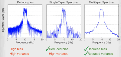
The plain periodogram - the FFT of finite data - is a poor spectral estimator: it has high variance (its value at neighboring frequency bins is nearly uncorrelated, giving a very noisy spectrum) and it is biased by leakage.
Split the signal into smaller (usually overlapping) windows.
Taper each window (e.g. Hanning) and compute its FFT / periodogram.
Average the power spectra of all chunks.
Averaging reduces the variance of the estimate roughly in proportion to the number of (partially independent) segments, and splitting makes the estimate less sensitive to non-stationarity and noise - at the price of reduced frequency resolution, because each chunk is shorter than the full recording.
Summary of the noise/resolution ladder:
no tapering (raw FFT of full data): highest resolution, but highest variance - very noisy spectrum
single-taper spectrum: less noise, but resolution limited by the main lobe
Welch averaging: much smoother, resolution limited by segment length
multitaper: best variance reduction at preserved resolution
psd_data.p contains powers, psd_data.f is the vector of frequencies.
The Gabor limit
There is a fundamental trade-off between time and frequency resolution - you cannot have both arbitrarily good (the uncertainty principle). Longer windows give finer frequency but coarser time resolution:
\[
\Delta t \, \Delta f \geq \frac{1}{4 \pi}
\]
narrow window: poor frequency resolution, good time resolution
wide window: good frequency resolution, poor time resolution
Practical rule of thumb: high-frequency components need good time resolution (they change quickly), while low-frequency components need good frequency resolution (they are spread widely in time). Wavelets formalize exactly this trade-off.
Morlet wavelet convolution
The STFT uses the same window at every frequency - fixed resolution everywhere. Wavelets fix this: a family of scaled versions of one basic shape, short at high frequencies and long at low ones, matching the Gabor limit to each band.
The Morlet (Gabor) wavelet is a complex sine tapered by a Gaussian:
psd_data.p contains powers, psd_data.f is the vector of frequencies.
Multitaper analysis
A single taper always throws signal away at the edges - attenuation that a single spectrum cannot recover. Multitaper analysis recovers it statistically:
The Fourier transform is computed several times, each time on data tapered with a different taper.
Each taper is multiplied element-wise with the signal, producing a windowed version from which one estimates power at each frequency.
Because each taper is pairwise orthogonal to the others, the resulting spectra are (approximately) statistically uncorrelated.
The final spectrum is the weighted average of all tapered spectra (eigenspectra).
Averaging \(K\) uncorrelated spectra reduces the variance by ~\(K\)-fold, while the combined tapers concentrate energy much better than any single taper could - recovering information that individual tapers lose to edge attenuation.
The tapers are Slepian functions / discrete prolate spheroidal sequences (DPSS), a family of orthogonal windows optimally concentrated within a chosen bandwidth \(NW\) (time-bandwidth product).
In NeuroAnalyzer:
psd_data =psd(eeg; ch = ["Fp1", "Fp2"], method =:mt, nt =16)
psd_data.p contains powers, psd_data.f is the vector of frequencies. nt is the number of tapers.
Adaptive weighting
Not all Slepian tapers are equally good: the \(k\)-th taper keeps a fraction \(\lambda_k\) (its concentration eigenvalue) of its energy inside the bandwidth \([-W, W]\), and the rest leaks in from distant frequencies. The first tapers have \(\lambda_k \approx 1\), the last usable ones noticeably less. With a plain average, this broadband leakage of the higher-order tapers fills the low-power parts of the spectrum with power leaked from strong peaks. This matters for EEG, whose 1/f spectrum spans many orders of magnitude: the high-frequency (e.g. gamma) power gets overestimated.
Thomson’s adaptive weighting fixes this by weighting each eigenspectrum \(\hat{S}_k(f)\) at each frequency by how much of it is likely to be true local power rather than leakage:
where \(\sigma^2\) is the signal variance. Because the weights depend on the unknown spectrum \(S(f)\), the two equations are iterated until convergence, starting from the average of the first two eigenspectra. Where the spectrum is high, all weights are ~1 and the estimate equals the plain average; where it is low, poorly concentrated tapers are down-weighted.
NeuroAnalyzer uses adaptive weighting by default (adaptive = true) for method = :mt. This applies to psd() and to all functions based on it (band_power(), plot_psd(), psd_slope(), etc.). To use the plain (equal-weight) average, as e.g. in DSP.mt_pgram():
p_ad, f =psd(eeg; ch ="Fp1", method =:mt, nt =16, db =true)p_eq, _ =psd(eeg; ch ="Fp1", method =:mt, nt =16, db =true, adaptive =false)fig =Figure(size = fig_size)ax =Axis(fig[1, 1]; xlabel ="Frequency [Hz]", ylabel ="Power [dB]")lines!(ax, f, p_eq[1, :, 1]; label ="equal weights")lines!(ax, f, p_ad[1, :, 1]; label ="adaptive weights")axislegend(ax)fig
The two estimates agree around the spectral peaks. In the low-power (high-frequency) range, the adaptive estimate is lower because the leakage is removed. The weighting costs very little time; turn it off only to reproduce results from other software that averages the eigenspectra with equal weights.
Choosing the number of tapers
The number of usable tapers is set by the time-bandwidth product: for a segment of duration \(T\) (seconds) and a spectral resolution (bandwidth) \(df = 2W\) (Hz, where \(W\) is the half-bandwidth), the number of well-concentrated tapers is \(K = 2TW - 1 = T \cdot df - 1\).
ntapers() returns this number for the epoch length of an object (floor(df × T) − 1, at least 1); df is the desired frequency resolution in Hz, i.e. the minimum separation between resolvable frequency peaks. For 10-second epochs:
for df in [2, 1, 0.5]println("df = ", df, " Hz: ", ntapers(e10; df = df), " tapers")end
Note the trade-off: smaller df (finer resolution) → fewer tapers → noisier spectrum; larger df → more tapers → smoother spectrum but coarser resolution.
Gaussian-filter Hilbert spectrogram
An alternative to the STFT for building a time-frequency representation, based on narrowband filtering and the Hilbert transform (which gives the instantaneous amplitude and phase of a narrowband signal):
Start from the time-domain signal.
Compute its FFT.
Multiply the spectrum by a Gaussian window centered at a specific frequency (a Gaussian filter, whose width sets the frequency resolution).
Compute the inverse FFT → the signal band-passed around that frequency.
Take the magnitude of the Hilbert transform (the analytic signal envelope) of the filtered signal: one row of the spectrogram - the amplitude over time at this specific frequency.
Repeat for all frequencies of interest.
The result is a smooth time-frequency amplitude map. Because the Gaussian filter has no side lobes, this method produces very clean, leakage-free representations; the trade-off is again the Gabor limit - the filter width in frequency fixes the temporal smear via \(\Delta t \, \Delta f \geq 1/(4\pi)\).
band_mpower() returns the mean band power (mbp), the frequency of the maximum power within the band (maxfrq), and the power (maxbp) and amplitude (maxba) at that frequency. The frequency of the maximum power in the beta band in 10-second epochs (first epoch):
mp =band_mpower(e10; ch ="eeg", flim =band_frq(e10; band =:beta))plot_bar(mp.maxfrq[:, 1]; glabels =labels(e10), xlabel ="Channels", ylabel ="Frequency [Hz]", title ="Frequency of maximum β power, epoch 1")
The posterior dominant rhythm of this recording is slow: its spectral peak is in the theta band rather than in the alpha band (see the PSD of O1 at the end of this tutorial). Frequency, power and amplitude at the peak of the 4–13 Hz range:
Tip: the maximum of a band is a true peak only if the spectrum has a local maximum within the band; without one (e.g. the alpha band of this recording), the maximum is at the lower edge of the band (8 Hz), because the power of the EEG decreases with frequency.
PSD slope
The power of the EEG decreases with frequency (approximately as \(1/f^\beta\), the aperiodic component). psd_slope() fits a straight line to the PSD (in dB, db = true) over the frequency range flim and returns the linear fit (lf), its slope (ls, in dB/Hz) and the frequencies of the fit (f):
flim = (1, 40)ps =psd(eeg; ch ="O1", db =true)sl =psd_slope(eeg; ch ="O1", flim = flim, db =true)f_idx =vsearch(flim[1], ps.f):vsearch(flim[2], ps.f)slope =round(sl.ls[1, 1]; digits =2)fig =Figure(size = fig_size)ax =Axis(fig[1, 1]; ax_style..., xlabel ="Frequency [Hz]", ylabel ="Power [dB]", title ="PSD of O1, slope = $slope dB/Hz")lines!(ax, ps.f[f_idx], ps.p[1, f_idx, 1]; color =:black)lines!(ax, sl.f, sl.lf[1, :, 1]; color =:red, linestyle =:dash)fig
Tip: a straight line on a linear frequency axis is a rough approximation of the aperiodic component; the FOOOF tutorial shows how to separate the aperiodic component from the oscillatory peaks.
Visualization
Plot Welch periodogram
plot_psd(eeg; ch ="Fp1")
Plot PSD, scale x-axis:
plot_psd(eeg; ch ="Fp1", frq =:log)
Plot Fast Fourier transform
plot_psd(eeg; ch ="Fp1", method =:fft)
Plot Short time Fourier transform
For PSD, short time Fourier transform is like the Welch’s method.
Plot short time Fourier transform PSD:
plot_psd(eeg; ch ="Fp1", method =:stft)
Plot Multi-taper
Plot multi-taper PSD:
plot_psd(eeg; ch ="Fp1", method =:mt)
The number of tapers can be set using ntapers(), where df is the required frequency resolution (the smallest distance between frequency peaks to be resolved, e.g. 1 Hz). plot_psd() shows a 10-second segment by default, so the number of tapers is calculated for 10-second epochs:
plot_psd(eeg; ch ="Fp1", method =:mt, nt =ntapers(e10; df =1))
In the interactive window, clicking on a PSD opens it enlarged in new window.
Plot Phase spectrum
Plot phase spectrum (one-sided FFT phase):
plot_phs(eeg;
         ch = ["Fp1", "Fp2", "F3", "F4"])
The phase of the ongoing EEG at each frequency is essentially random (uniformly distributed between −π and π), so the phase spectrum of a single segment looks like noise; phase becomes informative when it is compared between channels (phase differences, see the functional connectivity tutorials) or across trials (phase locking to an event).
Tip: the same plot types are available for plot_phs() as for plot_psd().
Plot band power in the δ, θ, α and β ranges
Frequency limits of the bands:
bands = [:delta, :theta, :alpha, :beta]frq = [band_frq(eeg; band = b) for b in bands]